

K-means clustering is a widely used unsupervised machine learning technique applied to seismic attributes for seismic facies classification. Traditional implementations of this method require the number of clusters (K) to be specified in advance. They can also suffer from the “initialization problem,” where poorly chosen starting cluster centers could lead to suboptimal solutions, and they offer limited intuitive visualization when dealing with high-dimensional data. A more modern variant, the Kmeans++ algorithm, addresses the initialization issue through a probabilistic “careful seeding” strategy that improves the likelihood of converging to a better clustering solution.
In this article, we explain these concepts in simple terms, discuss how these limitations can be mitigated, and demonstrate the use of this improved initialization along with methods for visualizing the resulting clusters. A “cluster” is a group of data points within a dataset that lie close to one another in feature space, and the process of partitioning a dataset into such groups is known as “clustering.” Identifying clusters is relatively straightforward in bivariate data; however, as the dimensionality of the data increases, recognizing and interpreting cluster structure becomes progressively more difficult.
The standard Kmeans clustering algorithm commonly used today was first introduced by Stuart Lloyd in 1957 while he was working at Bell Labs. Lloyd developed it as an iterative “least-squares quantization” method designed to minimize the average quantization noise power in pulse-code modulation for signal processing applications. Although the method was used internally for many years, it was not formally published until 1982.
The term “Kmeans” was later coined by James MacQueen to describe the process of partitioning N-dimensional data into K clusters. In this context, “K” is an integer specified in advance that represents the number of clusters expected in the dataset. The word “means” refers to the arithmetic averaging used to compute the centroid of each cluster, the average position of all data points assigned to that group.
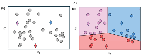
K=3 clusters. (b) In iteration 1, the three diamond-shaped points indicate the initial seed points. (c) We compute the distance of each data
point to each of the current cluster centers and assign each point to the cluster of the nearest one (colored regions).(d) In iteration 2,
the centroids (vector mean) of the three
clusters in (c) are recomputed, and their
positions are relocated (indicated by the
small arrows). (e) The distribution of data
points within each cluster is adjusted
based on the updated centroids, as shown
in (d). (f) In iteration 3, we compute new
centroids (vector means) from figure (e)
and indicate the updated locations by
arrows. (g) The data points are once more
reassigned to the closest cluster center.
This process continues iteratively until the
data points no longer shift. (Modified from
figure 2 of Galvis et al., 2017).
Lloyd’s method follows a “batch update approach” in which all samples (or voxels) are first assigned to their nearest cluster centers and the centroids are then updated. In contrast, MacQueen proposed an incremental (online) update method for the classification of multivariate observations, where cluster centers are updated as new data points are processed.
These developments were later extended in 2007 by David Arthur and Sergei Vassilvitskii, who introduced Kmeans++ to address the initialization problem of the standard Kmeans algorithm. Rather than selecting initial centroids randomly, Kmeans++ uses a probabilistic “careful seeding” strategy that spreads the initial centers more effectively across the data space, significantly improving both the speed of convergence and the quality of the final clustering results.
Classical Kmeans
The classical Kmeans clustering procedure begins by selecting K cluster centers, ck. These centers may be initialized either by placing them uniformly across the N-dimensional feature space or by randomly selecting K data samples from the dataset. Once initialized, Lloyd’s Kmeans algorithm proceeds through the following iterative steps:
- Compute the Euclidean distance between each data vector and all K centroids. Each data vector is then assigned to the cluster whose centroid is closest. The centroids remain fixed until all data points have been assigned to clusters.
- For each cluster, compute the mean vector of all data points assigned to it. This average becomes the new centroid for that cluster. The process is repeated for all K clusters, thereby updating the cluster centers.
- Determine whether the algorithm has converged (i.e., the cluster assignments or centroids no longer change significantly). If not, repeat the assignment and update steps until convergence is achieved or the changes become negligible.
Classical Kmeans++
The Kmeans++ algorithm improves cluster initialization by using a more careful seeding strategy based on the distances between data points. The process begins by selecting a random data sample and designating it as the first cluster center, c1. Next, the normalized squared distance between this center and all other data vectors is computed. The data vector with the largest normalized distance from c1 is then chosen as the second cluster center, c2. To determine the next center, the points corresponding to c1 and c2 are removed from the candidate list. The normalized distances between c2 and the remaining data samples are then calculated, and the point with the largest normalized distance is selected as the third cluster center, c3. This distance-based selection process is repeated iteratively until K distinct cluster centers have been established.
Once the initialization phase is complete, the procedure proceeds with the classical Kmeans clustering workflow introduced by Stuart Lloyd. In this stage, data vectors are assigned to the nearest cluster center, and the centroids are updated iteratively until the algorithm converges. By employing this careful seeding strategy, David Arthur and Sergei Vassilvitskii demonstrated that the method significantly improves the quality and stability of the clustering solution compared with classical random initialization.
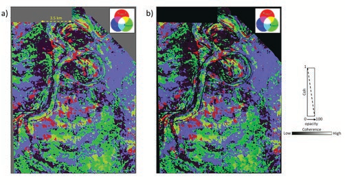
above a tracked marker extracted from
an RGB co-blended PCKmeans -1, PCKmeans -2
and PCKmeans -3 volumes. The different
colors on the display represent the seismic
facies at this level. (b)The same display as
in (a) but co-rendered with energy ratio
multispectral coherence. Fourteen of the
16 input attributes for Kmeans clustering used
logarithmic normalization. Unless noted
otherwise, all data courtesy NZP&M.
The above sequence of steps, applied to a dataset in which the points are not clearly separated into distinct clusters, is illustrated in figure 1.
One advantage of the K-means method is that it is computationally fast and straightforward to understand and implement.
The Distance Metric: Euclidean and Mahalanobis
The distance calculations discussed above between the centroid and the data points are based on the traditional Euclidean distance, which assumes that the classification variables are uncorrelated. When this assumption holds, clusters tend to appear spherical in crossplot space. In many practical situations, however, this assumption is not valid. Classification variables are often correlated, and the resulting clusters appear elliptical rather than spherical. In such cases, the traditional Kmeans method may perform poorly and might not converge to an optimal solution.
A more appropriate distance metric in the presence of correlated variables is the Mahalanobis distance, which accounts for the covariance structure of the data. However, this option is not always available in many commercial software implementations.
An alternative way to address this issue is to measure distances in an orthogonal Principal Component Analysis space (discussed earlier in the January 2022 installment of Geophysical Corner) rather than using Euclidean distance in the original, potentially correlated attribute space. By transforming the data into principal component space, the variables become uncorrelated, allowing the Kmeans algorithm to more effectively classify non-spherical and non-homogeneous clusters, as discussed below.
Visualization of Kmeans Clustering Output
More than 15 years ago, in a study carried out by Marcilio Matos and his coauthors, it was pointed out that results from Self-Organizing Mapping, discussed in several of our earlier articles, including the November 2020, January 2022, and June 2025 installments of Geophysical Corner, are commonly displayed using a rainbow color bar. They noted that this type of color mapping can obscure the underlying statistical and geological relationships among clusters.
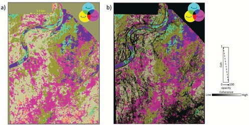
above a tracked marker extracted from
an CMY co-blended PCKmeans -1, PCKmeans -2
and PCKmeans -3 volumes. The different
colors on the display represent the seismic
facies at this level. (b) The same display as
in (a) but co-rendered with energy ratio
multispectral coherence. Fourteen of the
16 input attributes for Kmeans clustering used
logarithmic normalization.
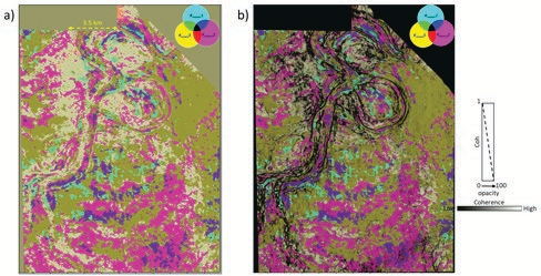
above a tracked marker extracted from
an CMY coblended PCKmeans–1, PCKmeans -2
and PCKmeans -3 volumes. The different
colors on the display represent the seismic
facies at this level. (b)The same display
as in (a) but corendered with energy ratio
multispectral coherence. Fourteen of the
16 input attributes for Kmeans clustering used
logarithmic normalization.
Instead, they proposed projecting the cluster prototype vectors (centroids) onto the first three components derived from PCA and co-rendering them using RGB colors. This provides a mathematically consistent method for visualizing high-dimensional data. With this projection-based color scheme, similarity in attribute space is reflected as visual similarity on the facies map. In other words, samples that are close in seismic attribute space appear as similar colors, producing a smooth and gradational palette. Subtle variations in color correspond to subtle differences in seismic waveforms or attributes, helping reveal stratigraphic continuity rather than imposing artificial boundaries.
The authors further demonstrated that this approach helps address the long-standing challenge of selecting the optimal number of clusters. By deliberately using more clusters than might be strictly necessary, statistically similar or redundant clusters are mapped to nearly identical colors through the PCA-to-RGB transformation. Consequently, these clusters visually merge (or “clump”) in the final display, reducing the interpreter’s dependence on precisely determining the value of K. In this way, combining multi-attribute clustering with topologically informed color mapping can significantly improve the delineation of complex geological features, such as turbidite channels, providing greater precision and geological consistency than conventional visualization techniques.
Application of Kmeans Clustering
In the June 2025 Geophysical Corner, we discussed two unsupervised machine learning techniques, namely PCA and SOM, applied to the Pipeline 3-D seismic survey from New Zealand. The objective was to identify architectural elements and discriminate seismic facies within a deepwater channel complex mapped at two different levels in two-way travel time. The study demonstrated that these machine learning approaches enhance spatial resolution and thereby assist seismic interpretation. Several attribute volumes were used, including relative acoustic impedance, gray-level co-occurrence matrix (GLCM) homogeneity, sweetness, peak magnitude, average frequency, and spectral magnitudes at frequencies ranging from 20 to 70 hertz in increments of 5 hertz.
In this case study, most of the attribute distributions were found to be skewed; only GLCM energy and relative acoustic impedance exhibited near-symmetric distributions. Because simple z-score normalization does not correct for skewness or kurtosis in the input data, we applied a logarithmic transformation to the attributes so that their distributions more closely approximated a Gaussian form. Additional details regarding the shapes of the individual attribute histograms using both z-score normalization and logarithmic transformation were presented in that article.
The same set of attributes is used here for the computation of Kmeans clustering.
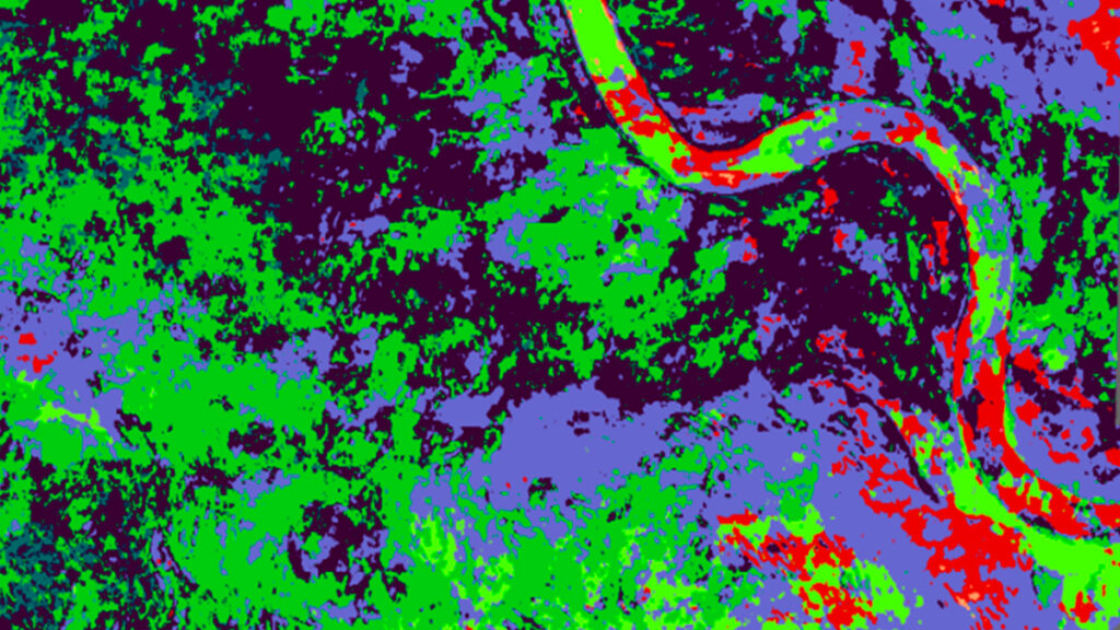
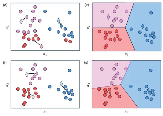
Figure 2a shows a horizon slice located 120 milliseconds above a tracked marker, extracted from an RGB co-blended volume composed of PCK1means , PCK2means, and PCK3means . The different colors represent distinct seismic facies at this level. Within the main channel, visible in the upper left portion of the display, several facies variations can be observed. Figure 2b shows the same slice co-rendered with energy-ratio multispectral coherence, which helps highlight the definition of the channel and other structural or stratigraphic features. The concept of RGB color blending was explained in detail in our December 2019 Geophysical Corner article.
A similar pair of displays, taken at 208 milliseconds above a tracked marker, is shown in figure 3. These images clearly delineate the channel geometry and the seismic facies variations within the main channel, as well as additional facies changes indicated by the arrows.
Both sets of displays appear somewhat dark due to the RGB co-blending. To improve visibility, we generated equivalent displays using CMY color blending. The resulting images, shown in figures 4 and 5, appear brighter overall, with color variations and geological features more clearly defined. As noted earlier, the CMY color-blending technique was also described in detail in our December 2019 Geophysical Corner article.
Conclusions
The evolution from Kmeans to the K ++ “careful seeding” technique provides a more stable and reproducible workflow for seismic facies classification. Although Euclidean distance is commonly used in clustering, applying the Mahalanobis distance or performing clustering in an orthogonal space derived from PCA better accounts for correlations among attributes and helps avoid the spherical bias that can arise when clusters are elliptical or irregular in shape. Because such advanced distance metrics are often unavailable in many commercial software packages, we advocate a visualization strategy that replaces arbitrary rainbow color bars with PCA-driven RGB co-rendering.
By projecting high-dimensional cluster centroids onto the first three principal components and mapping them to RGB colors, statistical similarity in attribute space is translated directly into visual similarity. This relational color mapping preserves stratigraphic continuity and naturally groups statistically similar clusters together. When combined with appropriate data normalization, the PCA–RGB approach provides a robust and practical framework that enhances the geological interpretability of multi-attribute seismic volumes.
Acknowledgements: The first author would also like to thank the Attribute Assisted Seismic Processing and Interpretation Consortium, University of Oklahoma, for access to their software, which has been used for all attribute computations. e