



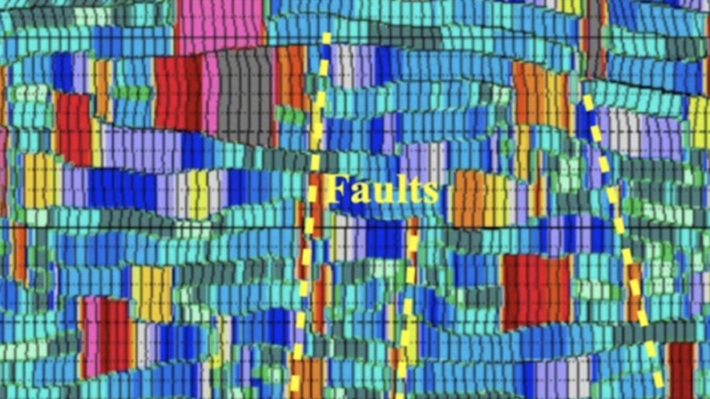
Most geoscientists are familiar with isochrons as measures of thickness, or as a time interval between two interpreted horizons. Traditionally, an isochron is viewed as a numerical representation of how much section sits between a peak and a trough, with little attention paid to whether that value is positive or negative. In practice, it is often treated as just another thickness measurement that records the separation between seismic events, even though a fault block might tilt one way or another.
However, what if the sign of the isochron measurement – positive or negative – contains meaningful geological information? This concept forms the basis of the signed-isochron, an attribute generated automatically as part of the distance-quadrant seismic attribute workflow (see the May 2025 Geophysical Corner). While the idea of assigning a polarity to an isochron measurement might seem straightforward, it introduces an additional layer of information that has largely been ignored in conventional seismic attributes and machine-learning workflows. By assigning a sign as an integral component of the measurement, the signed-isochron reveals subtle relationships and patterns that could otherwise remain hidden, opening new possibilities for seismic interpretation and subsurface characterization.
A Familiar Measurement, Recast
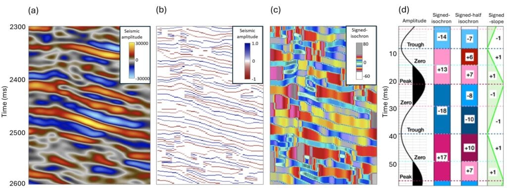
The DQ workflow begins by locating every peak, trough, and zero-crossing on a near-stack section. The near-stack data are preferred because they retain the higher frequency content needed to resolve thin, laterally continuous geological boundaries. The interpreted event times are written into an intermediate volume known as a StickOgram (Figure 1b), which itself is a useful product for horizon auto-tracking and fault interpretation.
The StickOgram naturally yields two isochron-type attributes. The conventional isochron is derived from peak-to-peak and trough-to-trough time intervals, while the half-isochron incorporates the zero-crossings, effectively doubling the vertical sampling density (Figure 1d). The final step is what gives the attribute its name. For each interval, the slope of the waveform is evaluated: intervals associated with rising waveforms are assigned positive values, while those associated with falling waveforms are assigned negative values. The resulting signed-isochron (Figure 1c) captures both interval thickness and polarity information and is available from the outset of a project, even before horizons or faults have been interpreted.
Reading the Sign on Real Data
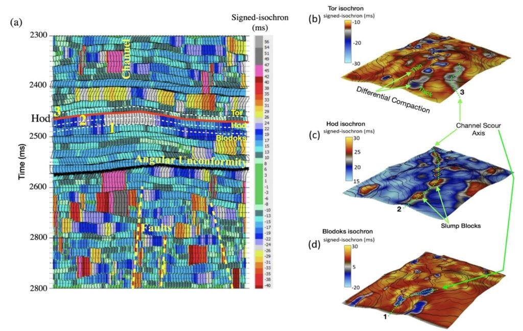
Figure 2a shows the signed isochron along a seismic line from the Volve Field, which is located in the southern Norwegian North Sea on the continental shelf. Above approximately 2,400 milliseconds, within the channelized Paleogene section, the continuous sand layers are characterized by positive isochron values, while the channels themselves show up appear as high-amplitude negative values. Between 2,400 and 2,500 milliseconds, the chalk interval is seen as more homogeneous, which fits the slow accumulation of coccolith material, though channel-negative anomalies are still visible within this interval.
Below approximately 2,550 milliseconds, an angular unconformity appears as a pattern of thinning and thickening across several layers. This surface corresponds to the truncation of oil sands along the southeastern flank of the structure. Beneath that unconformity, deformation associated with salt diapirism partitions the section into fault blocks, each internally consistent in its isochron values. Fault planes themselves often show up as narrow, laterally restricted anomalies. This is not surprising, since high-impedance boundaries tend to be disrupted within fracture zones.
Draping the signed-isochron attribute over the Hod marker (figures 2b–c) allows an interpreter to read channel scour, slumping, and differential compaction directly off the attribute. The point worth noting is the timing. This information is available prior to the final fault and horizon interpretation, allowing it to guide interpretation workflows rather than serve solely as a post-interpretation validation tool.
The Attribute Most ML Workflows Skip
Here is the puzzle: isochron-type measurements have been central to petrophysical inversion for decades. Furthermore, wedge models have long demonstrated how seismic amplitude and waveform shape change as a function of bed thickness across a wide range of porosity and fluid saturation values. Yet, the isochron, and especially the half isochron, is almost always absent from the standard list of ML input attributes. That standard list, which typically includes instantaneous amplitude, RMS amplitude, instantaneous frequency and phase, sweetness, and coherence, is built from continuous, sample-by-sample functions of a single seismic trace.
The isochron, however, is built differently, relying on discrete, event-to-event measurements. Its sample values come in step-like runs. Fifteen samples might all read the same 15-milliseconds value, then jump abruptly to a different constant. The signed-isochron amplifies this behavior by alternating between positive and negative step sequences (figure 2a). When fed into a standard feature-ranking process based on trend-fitting and R², this step pattern looks like noise and gets dropped early. The very thing that makes the isochron geologically meaningful – its abrupt, signed jumps – is what makes it statistically unattractive to conventional ranking processes.
Putting the Sign to Work
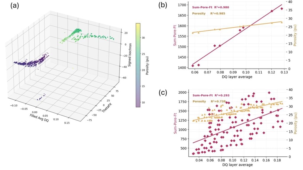
Rather than feeding the signed-isochron into a regression model alongside all the other attributes, we utilized it, first, as a discriminator to split the dataset before any trend-fitting happens. Figure 3a shows a 3-D crossplot of three DQ-derived attributes (DQ amplitude, ThetaPX gradient, and the signed-isochron) generated for a hidden-model dataset of 60 synthetic wells, each containing two distinct sand bodies. In this dataset, the sign of the isochron provides much of the separation between the two populations visible in the crossplot.
This interpretation is consistent with the underlying rock physics. In a typical sand-shale sequence, a medium- to high-amplitude peak corresponds to a soft-over-hard acoustic impedance boundary. The subsequent trough usually marks a hard layer terminating against a softer underlying formation. This sequence represents an alternation in waveform slope, which is precisely what the sign component is built to capture. In the siliciclastic, two-lithology settings examined so far, with relatively homogeneous shales and sands above roughly 20-percent porosity, this pattern has held up well. However, we anticipate that this relationship might be less clear in more heterogeneous or carbonate sections, which remain to be tested.
A second analytical pass on this subset, partitioning the data by isochron thickness, sharpens the results even further. Sum-pore-feet is the porosity-thickness product summed over the reservoir interval, a common proxy for storage capacity and a useful stand-in for porosity itself. When analyzing all the data points together (figure 3c), the R² for a sum-pore-feet trend is only 0.29. However, when the analysis is restricted to a narrow thickness window of approximately, 9.5–11 milliseconds (figure 3b), that metric climbs to 0.98, with the porosity fit reaching 0.985. The contrast between figures 3b and 3c effectively demonstrates the operational difference between a staged, sign-led workflow and a conventional merged-trendline approach.
Does It Show Up in the Prediction?
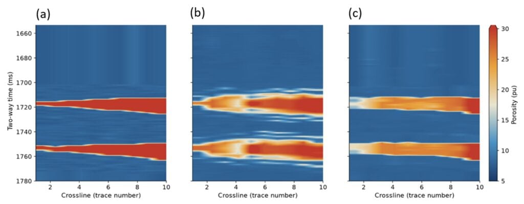
Figure 4 compares porosity predictions along a single line from a hidden-model dataset. A traditional instantaneous-attribute workflow, trained on the 13-well star, returns an R² value of only 0.32 when evaluated against the true porosity model (figures 4a versus 4b). In contrast, a workflow built around the signed-isochron significantly improves the R² to 0.70 (figure 4c). This optimized workflow first splits the data by sign, then partitions it by thickness before fitting porosity and pore-feet trends. While amplitude (DQ) and gradient (ThetaPX) still contribute to the final prediction, the staged integration of the sign component appears to be carrying much of the load.
A Caveat, and a Closing Thought
The results illustrated above come from one line of a synthetic, two-lithology operational dataset. The sign-based separation has so far been tested mainly in siliciclastic settings characterized by sands with porosities above 20 percent. Whether it holds up on field data with greater lithologic complexity, lower porosities, or carbonates is an open question, and one we plan to pursue as more datasets move through the DQ workflow.
Still, the basic lesson is worth keeping in mind: an attribute that looks like noise to a conventional feature-ranking step is not necessarily noise. Sometimes it just needs to go first.
Acknowledgements: The seismic data shown in figures 1 and 2 are from the Volve field, released to the public domain by Equinor and partners. We thank Equinor and the Volve license partners for making this dataset available for research and education.