


Seismic attributes ranging from RMS amplitude, through peak frequency, coherence, curvature, and impedance inversion are routinely applied to both accelerate and quantify the interpretation of 3-D time-migrated data volumes. In 2026, the ma
jority of deepwater 3-D seismic surveys are now prestack depth migrated. In addition, a significant number of recently acquired land 3-D seismic surveys are also prestack depth migrated, particularly when topography and complex overburden distort the target section of time-migrated images. Although these depth-migrated images are almost always superior to corresponding time-migrated images, many interpreters have been disappointed with the corresponding attributes, leading to the misperception that “attributes don’t work well on depth data.”
There are key differences between time- and depth-migrated images that can make attribute computation more challenging. We use a modern 3-D depth-migrated data volume from the Santos Basin, offshore Brazil, to illustrate how spectral balancing, structure-oriented filtering, and low-cut filtering to suppress steeply dipping events provide high-fidelity attribute volumes that can be used in both interactive interpretation and as input to machine learning
Seismic Attributes in Action
Seismic attributes measure patterns in the seismic data. The simplest attributes measure vertical patterns of amplitude, frequency, and phase along a seismic trace. Geometric attributes measure morphology patterns of dip, pinch out, continuity, curvature, and texture. Impedance attributes fall in between, and although applied to a single trace or gather, many algorithms include lateral constraints of a low-frequency model and/or inversion continuity. Although attributes are routinely used in mapping structure and stratigraphy, they are also useful in statistical analysis to predict seismic facies that may be more productive, pose drilling problems, or are more amenable to hydraulic fracturing. For example, Marcus Maas made a presentation in 2024 using prestack depth-migrated data in which he showed that in the Santos Basin of offshore Brazil, attributes used as input to machine learning could be used to differentiate porous limestone, tight limestone, hydrothermally altered dolomite, and igneous intrusives in a presalt environment. In his doctoral dissertation completed in 2025, he showed zones of exceptionally high flow rates (sweet spots) measured in sparse wells could be used to predict infill drilling targets. Post classification analysis showed that the hydrothermally altered dolomite facies exhibited low mean frequency, low bandwidth, negative curvature, and low coherence response. In what follows, we revisit one of these surveys and examine how to generate accurate attributes from depth-migrated data volumes.
Attribute Response of Depth-Migrated Data
The goal of this short article is to present a workflow that allows an interpreter to quantify the spectral response of depth-migrated data. Fortunately, almost all attributes work the same way on depth-migrated as on time-migrated data. Indeed, computing structural attributes such as vector dip (dip magnitude and azimuth) and curvature require the data to be in depth. If an interpreter first stretches their time-migrated to depth using well control or velocity analysis, they are in good shape, though the image might remain unfocused. However, if the interpreter computes dip (in degrees) and curvature, the software requires a simple (constant, and perhaps invariant between surveys) velocity to use to convert the data to depth. In general, depth-migrated data provide more accurate results, but with three caveats: First, depth migration provides excellent images in which time migration might fail. For this reason, a much larger percentage of depth-migrated volumes represent structural complexity, making the attribute interpretation process more challenging. Second, depth migration is designed to preserve steeply dipping events. These steep dips include not only stratigraphic reflections, but also fault-plane reflections and steeply dipping migration artifacts. Third, because of the change in velocity with lithology and depth, the seismic source wavelet is no longer “stochastic” – it changes its shape with location. For impedance inversion, a common practice is to vertically map the depth volume(s) back to time, perform the inversion process, and convert the results back to depth. For spectral analysis, the decomposition gives inaccurate results only at discrete, high-velocity contrast boundaries. Fortunately, these boundaries are provided by the velocity-depth model where spectral anomalies can be accounted for.
Spectral Balancing
For almost all interactive and quantitative interpretation, the ideal seismic spectrum should be flat, that is, the magnitude of the lowest, highest, and intermediate spectral components should exhibit nearly the same value. However, even with significant care, seismic sources and receivers exhibit only an approximately flat response, with seismic vibrators requiring long sweep times to impart more low frequency energy. Land data also suffer frequency variation from variable coupling to a heterogenous surface and irregular statics beneath the source and receiver arrays. For both land and marine data, intrinsic attenuation (for example, “squirting” fluids between pores as the seismic wave passes through) and geometric attenuation (scattering from rugose surfaces, for example) will attenuate higher frequencies more than lower frequencies.
A crude way to represent the spectral response is through the mean frequency and bandwidth. Although interpreters will often claim that they want “high-frequency” data, a more accurate wording would be that they want “high-bandwidth” data. Whereas the thinnest bed that can be mapped is determined by the highest frequency component, temporal resolution increases with the bandwidth.
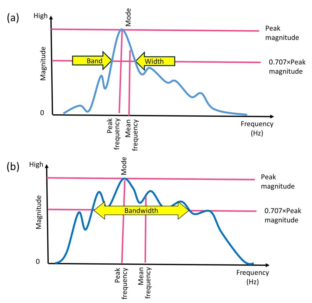
The parameters used in spectral balancing are computed, not from each trace, but rather from an average time-variant spectrum that represents the entire seismic survey. The result of spectral balancing is an average time-variant spectrum that is flat (see the March 2015 Geophysical Corner by Chopra and Marfurt). The impact of spectral balancing applied to an individual trace such as the cartoon in figure 1 broadens the spectrum but retains the tuning effects of variable layer thickness as well as localized attenuation anomalies. In figure 1, we define the peak magnitude, peak frequency, mean frequency, and bandwidth before and after spectral balancing. In this example, spectral balancing increases the value of the peak frequency, mean frequency, and the bandwidth.
Depth-Migrated Data and Low Wavenumbers (Long Wavelength) Components
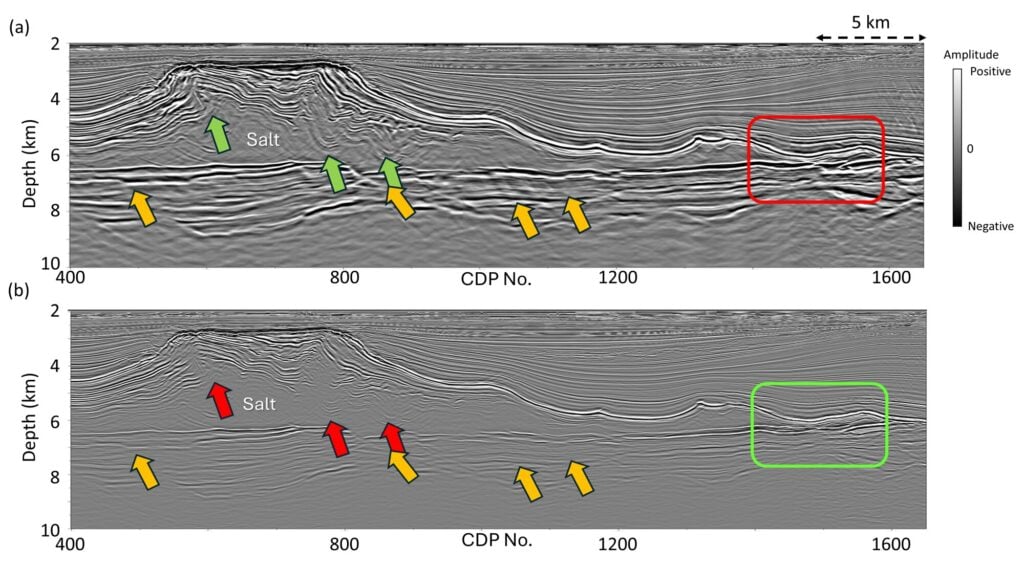
Figure 2a shows a representative vertical slice through the prestack reverse-time migrated Bacalhau survey acquired in the Santos Basin, offshore Brazil. There are three major units: (1) the shallower relatively low velocity Tertiary section, (2) the irregularly shaped, high velocity salt section in the middle, and (3) the deeper “presalt,” higher velocity carbonate and basalt/diabase section below about z=6.3 kilometers. The presalt exploration targets include porous carbonate buildups and hydrothermally altered dolomite. Green arrows indicate steeply dipping stratigraphic reflectors and the top of salt that have been accurately imaged by prestack depth migration. Prestack depth migration has also accurately imaged a suite of steeply dipping fault-plane reflections indicated by the orange arrows. In attribute analysis, as well as in impedance inversion, our goal is to enhance or quantify patterns in the stratigraphic reflections. If the fault-plane reflections overly or are juxtaposed to stratigraphic reflections, the attributes will map properties of the stronger event, not the one we want.
Interpreters are intimate with the concept of the apparent reservoir thickness measured by a vertical well traversing a steeply dipping reservoir, versus the true thickness measured perpendicular to the reservoir. The same issue appears in spectral decomposition, where we compute the spectral response along vertical seismic traces, not perpendicular to the reflectors. Steeply dipping events, whether stratigraphic, fault plane reflectors, or migration artifacts will appear in the lower-wavenumber part of the spectrum (a vertical event would have a wavenumber kz=0.0).
Figure 2b shows the same vertical section after spectral balancing and structure-oriented filtering followed by an Ormsby bandpass filter with corner wavenumbers of (3, 5, 40, 40) cycles/kilometer. Note the significant improvement in resolution between the red and green boxes. Balancing the low wavenumbers between 1 and 3 cycles/kilometer resulted in the fault-plane reflectors (and a few migration artifacts) being unacceptably strong. Orange arrows show that the undesired (for the attribute exercise, not for seismic mapping of faults!) indicated by the orange arrows have been suppressed. Unfortunately, the steeply stratigraphic reflectors indicated by the red arrows have also been removed. This is the kind of conundrum that seismic processors face every day – a filter that works well in one part of the data damages the data in a different part. The most common solution is to provide the interpreter with two volumes (one for structural and a second for stratigraphic interpretation, for example). Because our target is in the deeper presalt section, we can proceed with attribute analysis in this zone where the filter provides the desired result.
Structural Dip
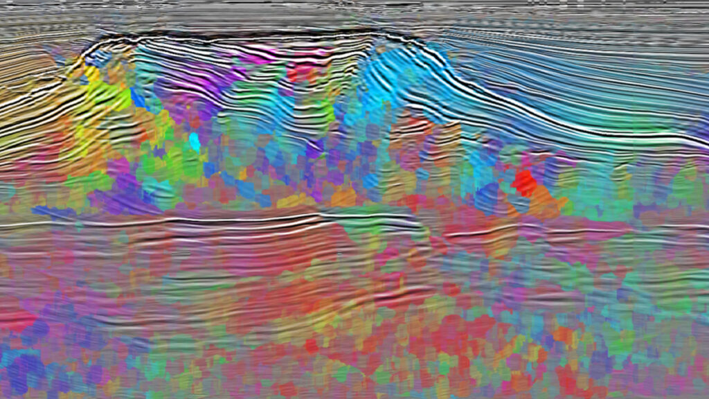
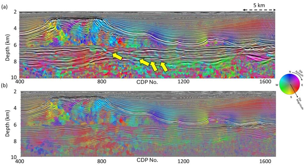
All geometric attributes (such as curvature, reflector convergence, coherence) as well as structure-oriented filtering require an accurate estimate of dip of the stratigraphic reflectors. If crosscutting and juxtaposed fault-plane reflectors or crosscutting migration artifacts are stronger than the stratigraphic reflectors of interest, we will compute the dip of the stronger (undesired) event. In the presalt section of the Bacalhau survey shown in figure 2, the application of the low-cut Ormsby filter reduces the contribution of the offending fault-plane reflections. Figure 3a show the corendered dip azimuth and dip magnitude (using a 2-D color wheel) computed from and corendered with the original data before spectral balancing. Note the laterally discontinuous vector dip estimates in the presalt section below z=6.3 kilometers. Yellow arrows indicate steeply dipping anomalies that represent the dip of fault-plane reflections rather than the dip of stratigraphic or igneous reflections. Figure 3b shows the vector dip computed from the data after spectral balancing followed by the low-cut Ormsby filter. The anomalous dips associated with the fault-plane reflections as well as steeply dipping migration artifacts are suppressed, providing a piecewise smoother vector dip image.
Results
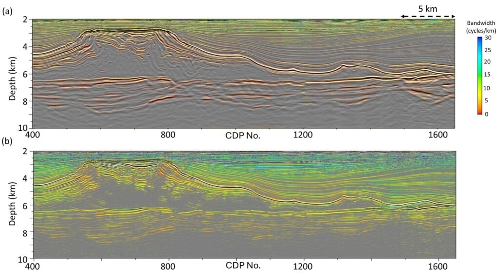
The most common estimates of the seismic spectrum are the mode (peak frequency), mean frequency, and bandwidth (see the July 2024 Geophysical Corner). The most commonly available estimates of these measures are based on complex trace analysis. Here, the peak frequency is approximated by the instantaneous frequency and the mean frequency by an envelope-weighted average of the instantaneous frequency. Figure 4a shows a vertical slice through the complex-trace generated mean frequency computed from the data without spectral balancing. In the Tertiary section about z=4 kilometers, the mean frequency is about 10 cycles/kilometer. In the target high-velocity presalt area below z=6.3 kilometers the mean frequency drops to about 5 cycles/kilometer. Figure 4b shows the same vertical slice but now generated using spectral decomposition computed from spectrally balanced amplitude volume. As stated earlier, spectral decomposition measures apparent spectral along the vertical trace axis. Because we now have the dip magnitude, , for each voxel shown in figure 3b, we can estimate the true dip as fTrue=fApparent/cos . In the Tertiary section about z=4 kilometers the spectral bandwidth is about 8 cycles/kilometer. Below z=6.3 kilometers the spectral bandwidth drops to about 3 cycles/kilometer. Figure 5b shows the same vertical slice but now generated using spectral decomposition (corrected for dip) computed from the spectrally balanced amplitude volume. In the Tertiary section about z=4 kilometers the spectral bandwidth is about 13 cycles/kilometer. In the faster target zone below z=6.3 kilometers the spectral bandwidth drops to about 8 cycles/kilometer, roughly doubling the range of the spectral response.
Conclusions
Prestack depth migration provides superior images in areas of complex structure and heterogeneous overburden, not only imaging steep dips but also correcting for velocity pullup, pushdown, and fault shadows seen in time-migrated images. Although seismic attributes work the same way on depth-migrated data as on time-migrated data, special care is required because attributes respond to the strongest seismic event within a given voxel. Consequently, the influence of steeply dipping fault-plane reflections and migration-related artifacts must be minimized to ensure reliable attribute interpretation. Spectral balancing also works the same way on depth-migrated data, providing higher bandwidth, higher resolution images that can be used in both interactive interpretation and as input to machine learning analysis.