

Seismic discontinuity attributes such as coherence and curvature are routinely applied to 3-D seismic data volumes to delineate faults or fractures, channel and reef edges, and other geological features. Such attributes are very helpful in interpretation, though the quality of the attributes generated depends on the quality of the seismic data in terms of coherent noise, incoherent noise and frequency content.
Once the 3-D seismic data reaches the interpreter’s workstation, it is presumed that the data have undergone optimal imaging and are free of processing artifacts such as multiples and over- and under-migration. We believe this to be true in most cases; and in those cases where it is not true, there is little the interpreter can do to correct the problem and the job becomes one of avoiding the interpretation of artifacts as geology. While the interpreter does not have the tools, expertise or time to reprocess seismic data, there are several steps that can be taken to precondition the data for subsequent attribute and impedance inversion analysis, some of which (such as structure-oriented filtering and trim statics) have been presented in this column over the last few years.
One of the more valuable data conditioning tasks is spectral balancing, or even enhancement, of the seismic data. Both of these processes need to be carried out carefully, with improvements in well ties to the seismic data, with well data being a critical validation step.
One of the processing strategies that may not be familiar to interpreters is to aggressively filter the data to facilitate a given process, but not to apply that filter in the final workflow. A classic example is to aggressively filter noise components to facilitate interactive velocity analysis. Once an accurate velocity analysis has been done, it is used to migrate the original (noise contaminated) rather than the filtered data, allowing migration to filter noise and enhance signal. We can do the same to precondition data for attribute analysis where we need to preserve edges, but not preserve amplitudes and phases.
Data Conditioning
Workflow for Coherence
We describe the sequential steps in data conditioning workflow for coherence as follows:
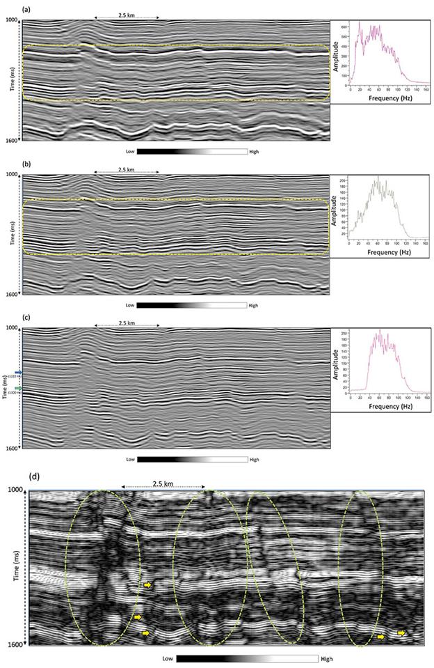
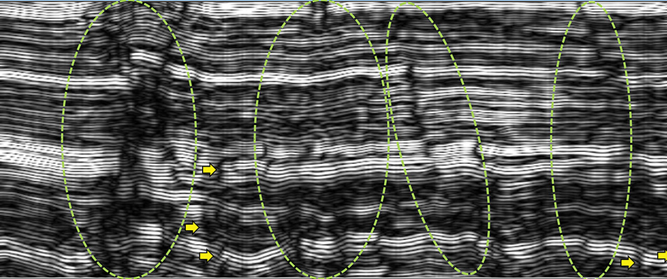
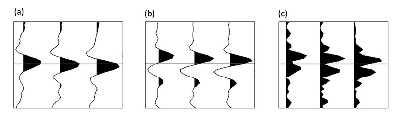
Figure 2: Vertical slices through the (a) seismic amplitude volume, (b) first derivative run on the seismic amplitude volume, (c) first derivative data in (b) band-pass filtered with a low cut of 40 Hz, and (d) absolute value of the band-pass filtered first derivative data volume in (c). Notice the somewhat higher resolution and detail on the display in (b), especially in the yellow highlighted portion. The higher frequency look is again more pronounced in the band-pass filtered display in (c). Finally, the discontinuities in the data appear to be enhanced on the absolute amplitude of first derivative display. Assuming that the input seismic data are preconditioned using structure-oriented filtering at the very least, one can compute the first derivative in almost any interpretation software package. The derivative does two things – it multiplies each frequency component by the frequency, f, resulting in spectral “bluing,” and it rotates the phase of the data by 90 degrees, so that the peaks and troughs of the amplitudes are transformed into zero crossings (figure 1b). In figure 2, we show a segment of a seismic section from the preconditioned input seismic data volume (figure 2a), and an equivalent section after computing the first derivative of this data (figure 2b). The average frequency spectra for the whole seismic volume and for the time window displayed are shown in the insets. Notice how the frequency spectrum shifts to the higher frequency side for the first derivative data. The first derivative data can be used as input to attributes such as coherence or curvature. If random noise has been previously suppressed by structure-oriented filtering, the resulting attributes often exhibit greater detail.
- If increasing the contribution of higher frequencies helps the coherence image, perhaps eliminating the low frequencies could help as well. We do so in figure 2c where we have applied a low-cut 40 Hz filter to the results shown in figure 2b, resulting in an image that appears to be of higher frequency.
- The previous two filters are linear. We might further extend the apparent frequency by taking the absolute value of each sample, or more simply, change all negative amplitude values to be positive. As seen in figure 2d we notice that the faults are defined much better, and the effect is seen equally well for structural or stratigraphic discontinuities.
Conclusion
The three processes above damage the true amplitude and phase of the data, and therefore cannot be used for subsequent impedance inversion or even simple bright spot analysis. However, these three filters do not significantly alter the location of discontinuities and of stratigraphic configuration.
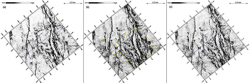
We demonstrate the value of such filtering by computing energy-ratio coherence attribute on the input, the data in step 2 (first derivative) and then the data in step 3 (first derivative with bandpass filter). Notice the improvement in continuity and resolution of the coherence anomalies (arrows in figure 3). All the steps mentioned earlier can be quickly carried out by an interpreter on a workstation with the available interpretation software package.
Like our processing analogy of velocity analysis, the interpreter now co-renders the improved coherence volumes with the original seismic data volume.